A Three Variable Macro Model : Estimation

We take simulated data from the three variable macro model in the last blogpost and try to estimate the parameters using Structural Vector Auto-Regression (SVAR). 

1. Graph, Summary Statistics & Correlations

Inflation is the annual increase in general prices measured in percentages. Nominal interest rates are also measured in % per annum. Output gap is usually calculated using some statistical filter (thus it has very small values). Typically a positive output gap implies that the economy demands for goods and services over and above its capacity. The quarterly data looks like this: 

Visually, the graph shows that inflation, interest rate and output gap are stationary. Stationarity means that the series is likely to have constant mean- Inflation always seems to return to 4%, interest rates to 6% and output gap to 0. Further, each series seems to have a constant variance - fluctuations do not get wider or narrower but remain even throughout.

We now look at the correlation between variables and their lagged values: 

Lets look closely at this matrix - each (i,j) entry in this matrix tells us the correlation of the i^th row entry with the j^th column entry. All variables are highly correlated with their own lags, indicative of strong persistence. Inflation & interest rates go hand in hand, while output gap moves against both of these variables. 

We go to our central bank’s website and find that it’s constitution says that “…our main endeavour will be to keep the general rise in consumer prices to 4% per annum…”. This means that the central bank was targeting inflation to be at 4%. The summary statistics confirm that inflation has been largely kept at the target of 4%. Further, nominal interest rates have been about 6% on average, which indicates that average real interest rates have been about 2%. This should correspond to the “natural” level of real interest rates - consistent with zero output gap. 

B. Structural Vector Auto Regression

Let us assume that the “structural” model is given by: 

The deltas form the constants in the regression, the gammas form the contemporaneous effects and the rest of the coefficients tell us how the variables are connected via lags. The “structural” shocks are independent of each other also. We cannot estimate the VAR in this form, we bring it to its “reduced form”:- 

After estimating the “reduced form” we need to go back to the “structural form”. This is the identification problem. If we compare equation (1) and (2) we see that: 

“Reduced form” shocks are not structural shocks but rather mixtures of structural shocks. There are many possibilities - output gap, inflation & interest rates all can effect each other contemporaneously - 6 free parameters (gammas). 

When we move from the estimated VAR parameters to the SVAR we need to restrict a few parameters to achieve identification. In this case we impose restrictions on at least 3 out of 6 of these contemporaneous effects. One plausible restriction is the Keynesian idea that firms don’t like to change prices that often and so inflation cannot respond immediately to output & interest rates. And sluggish output too does not respond to changed interest rates. This also fits well with the Monetarist idea that monetary policy suffers from transmission lags. In contrast, we allow inflation to effect output & interest rates without lag and output to effect interest rates without lag. So we impose: 

After this we deal with the question of how many lags. More lags means better fit but more parameters. The goal is to explain more with less. These criteria give us the lag order for which there is maximum goodness of fit with least parameters. The results say that a lag order of 1 makes most sense. 

We estimate the SVAR:

 Overall the model fit is excellent. But all contemporaneous effects are insignificant at 5 % level. Some lagged variables are insignificant at 5 % level. All those that were insignificant are force to zero in the final estimation. 

  The estimates change slightly, and one term that was earlier significant becomes insignificant (the effect of lagged output gap on interest rate becomes insignificant). The final estimates of parameters are given here:  

Further we can also say that inflation has a unit root. This corresponds well to the idea that expectations are adaptive. The final estimates also show that the central bank is indeed a pure inflation targeter. It does not seem to respond to output fluctuations. 

D. Impulse Response Function (IRFs)

The next step is to generate Impulse Response Functions (IRFs). These IRF plots tell us what structural shocks do to the economic system: 

1. Top row - positive ‘supply’ shock - purely to inflation: Pushes inflation above target immediately - the central bank responds a quarter later by raising interest rates. Rising inflation expectations, lowers real interest rates, which lead to a temporary positive output gap but that is quickly reversed because nominal interest rates have been raised. 
2. Middle row- positive ‘policy’ shock - purely to interest rates: leads to an immediate hike in interest rates which is quickly reversed, but which causes demand to fall in the next period and reduce inflation after another quarter. Interest rates are reversed, and through demand, bring inflation back up to target
3. Third row - positive demand shock - purely to output: which raises demand immediately. This has effect on inflation in the next quarter, which rises. And then interest rates rise in the 3rd quarter, to correct the rise in inflation.

Verdict

So did we get it right? Yes. All the coefficients were accurately identified, in terms of both direction and magnitude. And the Impulse Response Functions approximated the simulations carried out in the previous blog post. Just compare - 

The True Model :   

While this exercise was done in a very controlled environment we have demonstrated that advanced estimation techniques like the SVAR do work.

STATA codes to replicate, keep this irf file in working directory. 

A Three Variable Macro Model : Simulation

This blogpost shall simulate a simple 3 variable macroeconomic model of the business cycle. The first variable is the annual increase in general prices or inflation. The second is the “output-gap” which measures the log-difference between actual aggregate production and potential/full capacity GDP. It can also be thought of as a measure of excess demand for goods and services at the aggregate level. The third variable is the interest rate, which is the price of loans and credit in the economy, for both households and firms. 

These three variables are contenders for the most important variables in macroeconomics and influence each other over the business cycle. By simulation, I mean that I will run a virtual experiment. The system will start at rest, and I will introduce different types of ‘shocks’ at various locations, and then observe the dynamic movements of these three variables due to these shocks.

Since this is a purely imaginary economy, I make very simplifying assumptions and am in complete control over what is going on here. STATA Codes to replicate are at the end.

The Model

The following 5 equations fully describe the economy. One unit time in this tiny model economy is a quarter. 

Here (1) is the Aggregate Supply (AS) curve which says that inflation is a function of inflation expectations, output gap and supply shocks. Firms observing excess aggregate demand for goods and services will raise prices in the next quarter. Workers’ expectations of inflation influences how they negotiate for wages; higher the inflation expectations, the higher the wage negotiated. This leads firms to raise product prices. Supply shocks cover unpredicted changes in inflation due to oil prices movements, monsoon & climatic conditions in agriculture, etc.   

(2) is the dynamic Investment-Savings (IS) schedule that says that ex-ante real interest rates effect output gap with 1 quarter lag. Ex-ante real interest rates is defined in (3) and are nothing but interest rates in the same period minus inflation expectations for the next quarter; and measure the real price of credit & borrowing. 

If State Bank of India offers a home loan today, for an interest of 5%, a 10 lakh home will cost half a lakh in interest above the instalments for the principal. But if prices rise 5% tomorrow (and consequently your wage rises 5% with it), you will effectively end up paying zero interest for that loan! Therefore the ex-ante cost of credit depends on the interest rate today and the expectation of inflation tomorrow.

When the expected cost of credit is low consumers will execute plans take a home or car loans, investors and industrialists will take loans to invest in businesses. Therefore spending on goods and services will exceed the optimal capacity of the economy. However, transmission from interest rate to demand takes a full quarter.  

(2) Also says that at some price of credit (r*) the excess demand is zero. This is the “natural” rate of real interest rate, consistent with the economy’s capacity to produce. Apart from ex-ante real interest rates, we also have 𝜂_t which is the demand shock. This could consist of unpredictable changes in spending due to varying preferences for savings, changes in wealth caused by variations in asset prices, exchange rate fluctuations causing adjustments in exports & imports, abrupt movements in consumer and investor sentiment, etc.  

(4) is a Taylor rule, which describes how the central bank behaves. In our imaginary economy, the central bank’s sole mandate is to try and keep inflation at a target (𝜋*). It has control over the interest rate, because it is the banker to all commercial banks and at what rate it lends to them governs how they price credit. 

When inflation is on target (𝜋_t=𝜋*), the central bank keeps interest rates at r* + 𝜋*, so that (given inflation expectations are also equal to target), the ex-ante real interest rate is at its natural levels - and thereby there is no excess demand in the economy. If inflation is below its target, then the central bank lowers the interest rate below r* + 𝜋*. This raises the real interest rate, and according to (2) will create excess demand for goods and services. Excess demand will then, according to (1), raise inflation. The central bank will keep interest rates low until inflation is back on target. 

Apart from this, interest rates also changes due to policy shocks (v_t) which can arise due to frictions in transmission of monetary policy through commercial banks, or simply if the central bank decides to break from its rule of strict inflation targeting.  

(5) tells us that households, investors and workers always expect inflation to be what it was a quarter earlier. This is a very rudimentary rule of thumb, because obviously inflation will not be what it was a quarter earlier, because of changes in demand (whether caused by the central bank or by demand shocks) and supply shocks. Thus agents overlook the behaviour of firms and the central bank in determining inflation outcomes. But this is a simplifying assumption.

In summary: Monetary policy, is entirely concerned about inflation, effects aggregate demand through interest rates with one period lag and demand pressure generates inflation one period later. All three variables are interconnected, across time, to each other. And shocks intrinsic to each of them (demand, supply, policy) generate or power the dynamics in the economic system. 

Furthermore, we can describe the economic system in a more concise manner by solving (1) - (5) in terms of (𝜋_t,R_t,y_t)' the state vector, and writing in Vector notation: 

Stability of the system occurs when the state variables (𝜋_t,R_t,y_t) always tend to return to their steady-state values (𝜋*, r* + 𝜋*, 0) regardless of the magnitude of the shocks. This is assured only for certain ranges of parameter values (β, ϕ,θ), in all other cases the shocks whack the state variables permanently away from their steady state values. Stationarity occurs when the coefficient matrix of the lagged state vector is such - that it’s eigenvalues are within -1 and 1. We ensure this in the simulation. 

Simulations: Multiple Scenarios

We set the following parameters to be the following for the baseline case. The initial values for state variables are given to be their steady state values.

1. Demand, Supply & Policy Shocks 

First I introduce a positive supply shock of unit magnitude at quarter 5, which falls by 0.25 units every consecutive quarter till it reaches zero. What happens to the economy? The economy begins at steady state. Then in quarter 5, the supply impulse hits inflation, which rises above target. This has two effects in quarter 6. First, inflation expectations for quarter 6 rise. So anticipated real interest rate in quarter 6 falls. Thus demand rises in quarter 6, albeit temporarily. Second, the central bank responds to inflation overshooting target in quarter 5, by raising interest rates in quarter 6. This reverses the temporary increase in demand and causes a contraction in demand. This contraction in demand reduces inflation and brings it back to target levels. A negative supply shock, would reduce inflation first, then interest rates would fall after which demand would rise - restoring inflation back up to target levels. 

  

Next I introduce a positive demand shock at quarter 5, which also dies out like the  supply impulse. In this situation, it is demand which rises first in quarter 5 (a boom). This is followed by rising inflation in quarter 6, which has two effects - one, it further bolsters demand by raising inflation expectations and lowering real interest rates and two, it forces the central bank to swing into action in quarter 7. Interest rates thus respond last in this schemata, but are pivotal in bringing the economy back to target. A negative demand would do the reverse: lower demand, then lower inflation, which would have the central bank lower rates, which would reverse the recession and deflation.  

A similar positive policy shock is generated at quarter 5. So the central bank raises rates from in quarter 5, which it only gradually reduces. This reduces demand in quarter 6, which in turn, reduces inflation at quarter 7. Now the central bank must quickly reduce interest rates to bring inflation back up to target.

B. A Dovish Central Bank

The parameter ϕ tells us how hard the central bank reacts to inflation deviations from target, therefore it is a measure of how dovish or hawkish the central bank is. We reduce the value of ϕ to 1.2 and re-simulate the impulses. The key differences (a) the state variables, once disturbed, take much longer to get back to long run equilibrium. (b) the dovish central bank, by responding weakly, allows inflation to climb well above target.

   

C. Disinflation: Gradualist or Cold-Turkey

Here we simulate two different strategies to bring inflation to a lower target level. The goal of disinflation is to bring inflation down from 4% to 2%. The first approach is mild (call it “Gradualist”) while the other is aggressive (call it “Cold-Turkey”). 

 The Gradualist approach seeks to first reduce the target to 3% from quarter 5 onwards and then further reduce the target to 2% from quarter 25. I also keep the the central bank dovish by setting ϕ = 1.2. Cold-Turkey is when a hawkish central banker goes for immediate dis-inflation. In our simulation I re-set ϕ = 1.5 and have the central bank immediately begins to target inflation at 2% from quarter 5 onwards.   

What are the main differences? Gradualism takes a lot of time. Interest rates are not raised very high. It also does not push aggregate demand far below potential. In contrast, Cold-Turkey goes for heavy rate hikes that cause recession. This recession is used to disinflation the economy. Due to adaptive expectations, Cold-Turkey ends up creating serious output loss but achieves the task quicker than Gradualism. 

D. What a Dynamic Stochastic Economic System can look like

I re-simulate, bombarding the economy with random disturbances. The baseline parameters have been taken. The supply, demand and policy shocks that I have given are independent, identical and normally distributed with zero mean and certain variance. 

The resulting dynamics are complex and fascinating - shocks push the system away from its equilibrium but causal forces keep the system stable. 

Disclaimer - This is a purely imaginary economy. It borrows plot elements from the real world and plays out like a Bollywood movie. Any reference to any person or phenomenon, living or dead, is purely accidental and solely expositional!  

Why Simulate? 

1. it is expositional, gives clarity and visualisation
2. tells you what effect each parameter or shock has on the systems dynamics
3. since we built it, we can do whatever we like - we are the omnipresent and omniscient gods - we can explore ideas! 
4. is fun
5. helps test the power of estimation techniques - if estimation techniques are unable to figure out the parameters that were used to generate simulated data then they are probably not very useful against real world data

The next blogpost will cover (e) where we will using only this very simulated data, and see if empirical techniques called the Structural Vector Auto-Regression (SVAR) can get us back to square one i.e where we started from! 

Stata Commands to Replicate

What is Economic Geography?

The Nile

 Land and Man

Certain types of landforms are beneficial to society in many ways. For example, how a river can  help the economy depends on its stage of development. A young river is usually not safe for transport or navigation but  has great potential for generating power. A well-situated dam or hydraulic power pipe can greatly help the economy of that region. Hydropower is used for irrigation and for the operation of various mechanical devices, such as watermills, sawmills, textile mills, dock cranes, domestic lifts, powerhouses and in paint making. 

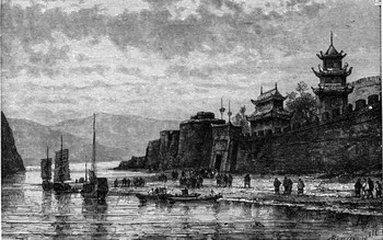
Similarly, a mature river does not have the force to generate electricity without incurring heavy cost for such energy, but does have the speed to allow navigation and transport. It also enables agricultural activities by making the soil more fertile. This allows for trade and commerce that greatly expands market activities and incomes together. Without the river Nile, the Egyptian civilization could not have flourished. The Nile brought vegetation, transport and agriculture upon which the Egyptians built their civilization. The Indus Valley Civilization was founded on the banks of many rivers - Jhelum, Chenab, Ravi, Satluj and Beas. The Chinese Yellow River Valley Civilization (4000BC) also grew around the Huange He river, which enabled agriculture.

 

Development along the Yellow River

Temperature changes are also an important factor that influences economic activity. There is a vast amount of literature that claims that hot areas have lesser economic activity and development. A recent study claims that in the poor countries, about 1 degree rise in temperature on an average causes about 1.3% fall in economic activity. Temperature changes can also lower agricultural and industrial output and indirectly impact political stability. The latitude, altitude and the relative distance to water bodies and landforms determine the climate of an area. In turn, the climate of an area determines the population and demography.

Even in today’s world, the Indian economy is sometimes called the ‘Monsoon Economy’ since it depends heavily on the seasonal winds that blow from the Indian Ocean and the Arabian Sea that bring heavy rains. This heavy rain in June and September has huge effect on the agriculture of India. The impact is such that if the monsoon is delayed by over a week then the Indian GDP growth slows down. Every year the country hopes for timely monsoons and a favourable weather.

Indian kids pray for rain

The rock formation of the land is also has a major influence on the economic activity. Rocks are  broadly categorised  into igneous, metamorphic and sedimentary rocks. Each category has further divisions and sub-divisions, and only some forms of rocks have economic value. Soils that originate from sedimentary rocks are generally more fertile and in particular if the soil is derived from limestone. There is a saying, 'A limestone country is a rich country'. In today's times ownership of large oil reserves can help the country become prosperous (or bring civil war!) for instance Canada or Syria. 

To try and understand how distances have played a large part in our evolution, we can take a look at the industrial revolution. Prior to this revolution, the most advanced civilizations of the world were in Asia. But once the industrial revolution set in, the West took over in innovation and production. This was characterized by two prominent features:

First, the incredible rise in average productivity and the outstanding leap into more efficient methods of production. As newer methods of producing goods and services sprang up, the productivity of the western world increased forty times in just a hundred years. The Cotton Gin, Sewing Machine, Diesel Engine and the famous Assembly Line made it much easier for the industries to be set up. 

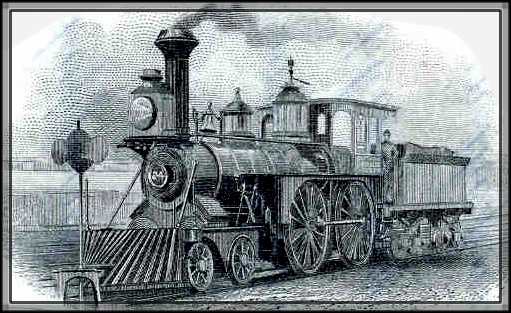
Second, the cost of transportation fell to almost a tenth of what it was. The invention of the steam engine and the aeroplane brought places and people much closer. The invention of the telegram made communication a thousand times faster than before. The area where goods were produced did not have to be close to people's homes anymore. Factories and industries came up further from the city where production multiplied rapidly. This tells us that transportation is extremely important for economic activity. 

Emergence of Cities

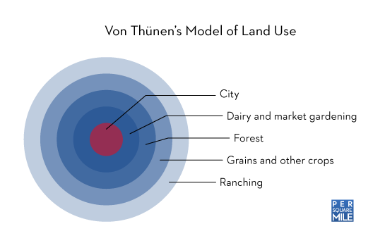
Urban Economics is the study of urban society. Economists use microeconomic tools to help understand crime, education, finance and other urban variables. Urban Economics attempts to incorporate distances and locations, into how cities develop. It began with Von Thunen and his work on how scarce resources are allocated as per locations in cities.

MONOCENTRIC CITIES

Imagine a circular city in a featureless plain. All employment is in a central business district (CBD), which we take to be a point at the city’s centre. All the workers live around the CBD and go to work every day. The further they live from the city, the costlier it will be to travel to work every day. However, the further they live from the city, the cheaper it is to get a place to stay. Each worker also purchases other goods and services that are important to them. In effect, the income the worker receives from the CBD is used in three ways,

·      Rent for housing services

·      Transport to the CBD and back

·      Purchase of other goods & services

This model claims that workers want to try and obtain as much housing services and other goods & services. And if the income obtained from the CBD is fixed, the worker must try and choose a home that is far enough to be cheap but at the same time close enough to the CBD to have low transport costs. The question that this model answers is ‘how far from the CBD does the worker choose to stay?’

The model also proceeds to answering the following questions, does the worker’s choice of residence change if: -

1)    The housing rents per unit distance from the CBD         change?

2)    The income obtained from the CBD changes?

3)    If the costs of other goods and services change?

4)    If there are frequent traffic jams in the city?

5)    If the travel costs change?

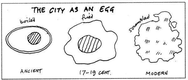
This city goes on to become even more complicated and tries to provide an explanation as to why cities expand and come up in the first place. Monocentric city models gave way to Polycentric city models. Cities are very complex things and we still have a lot to understand about them. 

Hotelling's Beach

This theory tries to understand how firms set up shops. It was developed under Harold Hotelling and tries to understand how the market arises. Sellers try to position themselves as far away from other sellers and as close to the buyers. We can see interesting patterns and designs in the way sellers behave. The theory incorporates a lot of ideas from Game Theory since the sellers use competitive strategies to try and maximize profit. We take the help of a simple illustration to explain Spatial Competition.

Hotelling’s Beach: Imagine a beautiful day at a beach. One can observe many people sitting in the sand, just relaxing. It’s a hot day and everyone really wants to have an ice cream. But, since the sand is really hot, no one really wants to walk a lot. They'd all prefer if the ice cream seller comes near them.

Along comes an ice cream seller and since she is early, she is the only seller in the market. Once she gets here, she has a problem. Where will she set up shop? The answer is that she will set up shop right in the centre, where people have less discomfort in getting up and reaching for the ice cream. This is the place where she can maximise her profits. 

Now the interesting change occurs when another seller joins her. Now in order to maximize profits they must adjust their locations so that they reach out to as many people as they can, within the competitive environment. The best possible scenario is when they divide the market share equally and adjust their locations to cater to two groups of consumers.

The theory goes on to explain what happens in situation when there are more and more sellers in a larger region. This theory is very evident in real life, especially in India where small shops are in plenty. From the locations of panipuri stalls to paan shops, we observe spatial competition.

The Economic Space

In most contemporary economic thought, geographical distances have been largely ignored. Transport costs have not been given much weightage and most economic theories consider transport costs to be zero. When the classical economists studied the economy, they considered the distances between cities, countries and people themselves to be irreverent. This is quite clear when the famous economist David Riccardo constructed his theory of ‘comparative advantage’ by first assuming that there was perfect mobility within countries. In a perfectly mobile environment, factors of production like labor and capital can move freely without difficulty. Most of the economists like Smith and Riccardo grew up in the British Empire. And since Britain had already established trade routes all over the world, they and their followers tended to ignore transport costs over the sea. Hence, most classical economic theories consider the world to be “upon the tip of a needle” as they all do not pay attention to space. Only a handful of mainstream economic theories such as Hotelling's Competition and Urban Economics, take the entire distances into consideration. 

The only spaces that economists regarded well were the national borders. Apart from this minor division of the world, economic theories did not look at the differences in landscape and terrain. And as once Samuelson said,

‘Spatial problems have been so neglected in economic theory that the field is of interest for its own sake.’

The concept of the economic space is needed because the prices of goods and services, the incentives of people and the decisions of firms depend on distances. As Debreu once said,

‘A good at a certain location and the same good at another location are different economic objects, and the specification of the location at which it will be available is essential.’

A good economic theory must always consider the economic space.

Insights 

Although Economic Geography is still very young compared to Macroeconomics or other mainstream economic theories, it has provided us with very valuable insights. These insights come from a study of the economic space in a  scientific manner. 

traffic jam

• Transportation Costs play a major role even in today's fast moving world. Globalisation has brought in a feeling that the world has become flat, but the truth is different. Physically, culturally and economically the world is still round. Distances and locations play a very important role in the modern economy.

• Factor Mobility or how easily labor and capital are moved to a desired location, is very important for the economy. Not only international mobility, but also national mobility matters. Economic Geography tells us that there is a growing divide between some people and others. This disparity of national mobility could pose a problem.

• International Trade is good for everyone. Economic Geography helps confirm the belief that trade beyond barriers is good for both parties. It helps enhance the diversity and variety of goods and services available to us. 

Geography is one of the most interesting subjects I ever encountered. I loved to study about glaciers, rock faces, erosion, deserts and vegetation. From the formation of stalactites and stalagmites to the corrosion caused by waves, the subject manages to capture one’s attention. It’s a very beautiful subject that made me imagine a lot. Economics on the other hand, focuses more on the human species. It studies the effects of consumption and saving. It tries to understand the meaning of money. And even though it may seem a bit drab, it has its elusive beauty.

It is a pleasure to incorporate the beauty of the earth and the complexity of human beings and study Economic Geography. This field has gained traction over the last few decades. The importance of transport costs and increasing returns has begun to invade modern economic thought in an entirely new way. We cannot hope to understand economic activity without understanding the economic space it exists in. It is a necessity to incorporate the geographical conditions when we want to apply economic models to real life, since real life has real differences in landscape.  There is much more to be done in this field and a lot to break through.

Economics is for everyone!

Geography is for everyone!